NLP Summary
ELMo
Introduction
Our word vectors are learned functions of the internal states of a deep bidirectional language model (biLM), which is pretrained on a large text corpus.
learning high quality representations can be challenging. They should ideally model both:
- complex characteristics of word use (e.g., syntax and semantics), and
- how these uses vary across linguistic contexts (i.e., to model polysemy).
ELMo (Embeddings from Language Models). ELMo representations are deep, in the sense that they are a function of all of the internal layers of the biLM.
Using intrinsic evaluations, we show that the higher-level LSTM states capture context-dependent aspects of word meaning (e.g., they can be used without modification to perform well on supervised word sense disambiguation tasks) while lowerlevel states model aspects of syntax (e.g., they can be used to do part-of-speech tagging).
Related work
Due to their ability to capture syntactic and semantic information of words from large scale unlabeled text, pretrained word vectors are a standard component of most state-of-the-art NLP architectures. However, these approaches for learning word vectors only allow a single contextindependent representation for each word.
Previously proposed methods overcome some of the shortcomings of traditional word vectors by either enriching them with subword information or learning separate vectors for each word sense. Our approach also benefits from subword units through the use of character convolutions, and we seamlessly incorporate multi-sense information into downstream tasks without explicitly training to predict predefined sense classes.
Other recent work has also focused on learning context-dependent representations. context2vec uses a bidirectional LSTM to encode the context around a pivot word. Other approaches for learning contextual embeddings include the pivot word itself in the representation and are computed with the encoder of either a supervised neural machine translation (MT) system or an unsupervised language model.
what?
Previous work has also shown that different layers of deep biRNNs encode different types of information.
ELMo: Embeddings from Language Models
ELMo word representations are functions of the entire input sentence. They are computed on top of two-layer biLMs with character convolutions, as a linear function of the internal network states. This setup allows us to do semi-supervised learning, where the biLM is pretrained at a large scale and easily incorporated into a wide range of existing neural NLP architectures.
Bidirectional language models
At each position k, each LSTM layer outputs a context-dependent representation h(LM, k, j) where j = 1,…,L. The top layer LSTM output, h(LM, k, L) , is used to predict the next token tk+1 with a Softmax layer.
A backward LM can be implemented in an analogous way to a forward LM, with each backward LSTM layer j in a L layer deep model producing representations h(LM, k, j) of tk given (tk+1,…,tN).
A biLM combines both a forward and backward LM. Our formulation jointly maximizes the log likelihood of the forward and backward directions:
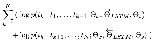
We tie the parameters for both the token representation (Θx) and Softmax layer (Θs) in the forward and backward direction while maintaining separate parameters for the LSTMs in each direction.
ELMo
ELMo is a task specific combination of the intermediate layer representations in the biLM. For each token tk, a L-layer biLM computes a set of 2L + 1 representations.
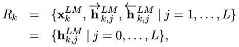
h(LM, k, j) is the token layer.
ELMo collapses all layers in R into a single vector, ELMok = E (Rk; Θe). More generally, we compute a task specific weighting of all biLM layers:
stask are softmax-normalized weights and the scalar parameter γtask allows the task model to scale the entire ELMo vector. γ is of practical importance to aid the optimization process.
Considering that the activations of each biLM layer have a different distribution, in some cases it also helped to apply layer normalization (Ba et al., 2016) to each biLM layer before weighting.
Using biLMs for supervised NLP tasks
To add ELMo to the supervised model, we first freeze the weights of the biLM and then concatenate the ELMo vector (ELMo, task, k) with xk and pass the ELMo enhanced representation [x; (ELMo, task, k)] into the task RNN.
Finally, we found it beneficial to add a moderate amount of dropout to ELMo and in some cases to regularize the ELMo weights by adding λ∥w∥2 to the loss. This imposes an inductive bias on the ELMo weights to stay close to an average of all biLM layers.
Pre-trained bidirectional language model architecture
For a purely character-based input representation, we halved all embedding and hidden dimensions from the single best model CNN-BIG-LSTM in Jozefowicz et al. (2016). The final model uses L = 2 biLSTM layers with 4096 units and 512 dimension projections and a residual connection from the first to second layer. The context insensitive type representation uses 2048 character n-gram convolutional filters followed by two highway layers (Srivastava et al., 2015) and a linear projection down to a 512 representation.
The context insensitive type representation uses 2048 character n-gram convolutional filters followed by two highway layers and a linear projection down to a 512 representation.
As a result, the biLM provides three layers of representations for each input token, including those outside the training set due to the purely character input.
Once pretrained, the biLM can compute representations for any task.
ULMFiT
Introduction
We propose Universal Language Model Fine-tuning (ULMFiT), an effective transfer learning method that can be applied to any task in NLP, and introduce techniques that are key for fine-tuning a language model.
transductive transfer vs. inductive transfer
what?
Language models (LM) overfit to small datasets and suffered catastrophic forgetting when fine-tuned with a classifier. Compared to CV, NLP models are typically more shallow and thus require different fine-tuning methods.
We propose a new method, Universal Language Model Fine-tuning (ULMFiT) that addresses these issues and enables robust inductive transfer learning for any NLP task.
The same 3-layer LSTM architecture— with the same hyperparameters and no additions other than tuned dropout hyperparameters— outperforms highly engineered models and trans-fer learning approaches on six widely studied text classification tasks.
Our contributions are the following:
- We propose Universal Language Model Fine-tuning (ULMFiT), a method that can be used to achieve CV-like transfer learning for any task for NLP.
- We propose discriminative fine-tuning, slanted triangular learning rates, and gradual unfreezing, novel techniques to retain previous knowledge and avoid catastrophic forgetting during fine-tuning.
- We significantly outperform the state-of-the-art on six representative text classification datasets, with an error reduction of 18-24% on the majority of datasets.
- We show that our method enables extremely sample-efficient transfer learning and perform an extensive ablation analysis.
Related work
Hypercolumns
The prevailing approach is to pretrain embeddings that capture additional context via other tasks. Embeddings at different levels are then used as features, concatenated either with the word embeddings or with the inputs at intermediate layers. This method is known as hypercolumns.
Universal Language Model Fine-tuning
We propose Universal Language Model Fine-tuning (ULMFiT), which pretrains a language model (LM) on a large general-domain corpus and fine-tunes it on the target task using novel techniques. The method is universal in the sense that it meets these practical criteria:
- It works across tasks varying in document size, number, and label type;
- it uses a single architecture and training process;
- it requires no custom feature engineering or preprocessing; and
- it does not require additional in-domain documents or labels.
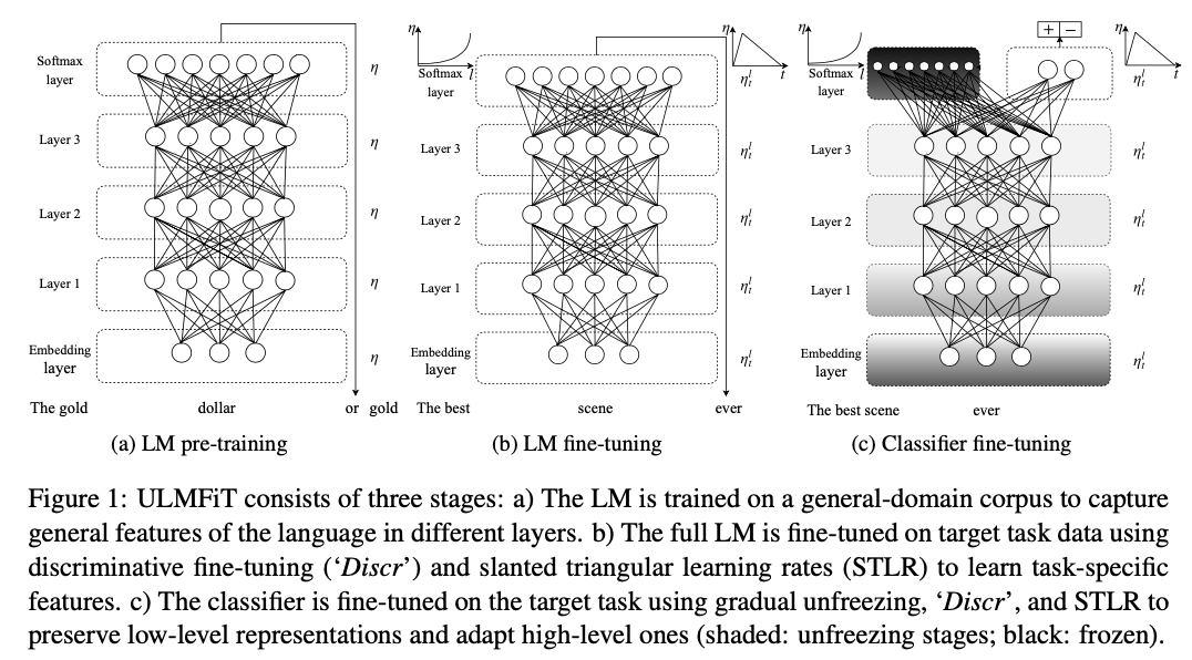
ULMFiT consists of the following steps, which we show in Figure 1: a) General-domain LM pretraining; b) target task LM fine-tuning; and c) target task classifier fine-tuning.
General-domain LM pretraining
We pretrain the language model on Wikitext-103 (Merity et al., 2017b) consisting of 28,595 preprocessed Wikipedia articles and 103 million words.
Target task LM fine-tuning
We thus fine-tune the LM on data of the target task. Given a pretrained general-domain LM, this stage converges faster as it only needs to adapt to the idiosyncrasies of the target data, and it allows us to train a robust LM even for small datasets. We propose discriminative fine-tuning and slanted triangular learning rates.
Discriminative fine-tuning
For discriminative fine-tuning, we split the parameters θ into {θ1, . . . , θL} where θl contains the parameters of the model at the l-th layer and L is the number of layers of the model. Similarly, we obtain {η1,…,ηL} where ηl is the learning rate of the l-th layer.
The SGD update with discriminative fine-tuning is then the following:
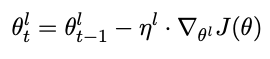
We empirically found it to work well to first choose the learning rate ηL of the last layer by fine-tuning only the last layer and using ηl−1 = ηl/2.6 as the learning rate for lower layers.
Slanted triangular learning rates
we propose slanted triangular learning rates (STLR), which first linearly increases the learning rate and then linearly decays it according to the following update schedule, which can be seen in:
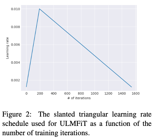
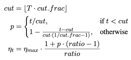
where T is the number of training iterations, cut_frac is the fraction of iterations we increase the LR, cut is the iteration when we switch from increasing to decreasing the LR, p is the fraction of the number of iterations we have increased or will decrease the LR respectively, ratio specifies how much smaller the lowest LR is from the maximum LR ηmax, and ηt is the learning rate at iteration t.
We generally use cut_frac = 0.1, ratio = 32 and ηmax = 0.01.
Target task classifier fine-tuning
Finally, for fine-tuning the classifier, we augment the pretrained language model with two additional linear blocks.
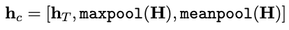
Concat pooling
As input documents can consist of hundreds of words, information may get lost if we only consider the last hidden state of the model. For this reason, we concatenate the hidden state at the last time step hT of the document with both the max-pooled and the mean-pooled representation of the hidden states over as many time steps as fit in GPU memory H = {h1,…,hT}:
Gradual unfreezing
We first unfreeze the last layer and fine-tune all unfrozen layers for one epoch. We then unfreeze the next lower frozen layer and repeat, until we finetune all layers until convergence at the last iteration.
BPTT for Text Classification (BPT3C)
In order to make fine-tuning a classifier for large documents feasible, we propose BPTT for Text Classification (BPT3C): We divide the document into fixedlength batches of size b. At the beginning of each batch, the model is initialized with the final state of the previous batch.
Bidirectional language model
For all our experiments, we pretrain both a forward and a backward LM.
Transformer
Introduction
Recurrent models typically factor computation along the symbol positions of the input and output sequences. Aligning the positions to steps in computation time, they generate a sequence of hidden states ht, as a function of the previous hidden state ht−1 and the input for position t.
This inherently sequential nature precludes parallelization within training examples, which becomes critical at longer sequence lengths, as memory constraints limit batching across examples.
Attention mechanisms have become an integral part of compelling sequence modeling and transduction models in various tasks, allowing modeling of dependencies without regard to their distance in the input or output sequences
In this work we propose the Transformer, a model architecture eschewing recurrence and instead relying entirely on an attention mechanism to draw global dependencies between input and output.
Background
The goal of reducing sequential computation also forms the foundation of the Extended Neural GPU [20], ByteNet [15] and ConvS2S [8], all of which use convolutional neural networks as basic building block, computing hidden representations in parallel for all input and output positions.
In these models, the number of operations required to relate signals from two arbitrary input or output positions grows in the distance between positions, linearly for ConvS2S and logarithmically for ByteNet. This makes it more difficult to learn dependencies between distant positions.
In the Transformer this is reduced to a constant number of operations, albeit at the cost of reduced effective resolution due to averaging attention-weighted positions, an effect we counteract with Multi-Head Attention.
Self-attention, sometimes called intra-attention is an attention mechanism relating different positions of a single sequence in order to compute a representation of the sequence.
To the best of our knowledge, however, the Transformer is the first transduction model relying
entirely on self-attention to compute representations of its input and output without using sequencealigned
RNNs or convolution.
Model Architecture
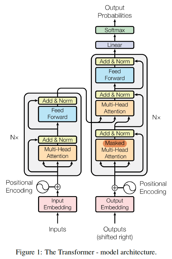
The Transformer follows this overall architecture using stacked self-attention and point-wise, fully connected layers for both the encoder and decoder, shown in the left and right halves of Figure:
Encoder and Decoder Stacks
Encoder:
The encoder is composed of a stack of N = 6 identical layers. Each layer has two sub-layers. The first is a multi-head self-attention mechanism, and the second is a simple, position-wise fully connected feed-forward network.
We employ a residual connection around each of the two sub-layers, followed by layer normalization. That is, the output of each sub-layer is LayerNorm(x + Sublayer(x)), where Sublayer(x) is the function implemented by the sub-layer itself.
To facilitate these residual connections, all sub-layers in the model, as well as the embedding layers, produce outputs of dimension dmodel = 512.
Decoder:
The decoder is also composed of a stack of N = 6 identical layers. In addition to the two sub-layers in each encoder layer, the decoder inserts a third sub-layer, which performs multi-head attention over the output of the encoder stack.
Similar to the encoder, we employ residual connections around each of the sub-layers, followed by layer normalization.
We also modify the self-attention sub-layer(Masked Multi-Head Attention) in the decoder stack to ensure that the predictions for position i can depend only on the known outputs at positions less than i.
Attention
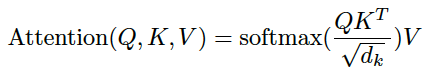
An attention function can be described as mapping a query and a set of key-value pairs to an output, where the query, keys, values, and output are all vectors. The output is computed as a weighted sum of the values, where the weight assigned to each value is computed by a compatibility function of the query with the corresponding key.
Attention(Q, K, V) = softmax(Q * K.T / √dk) * V
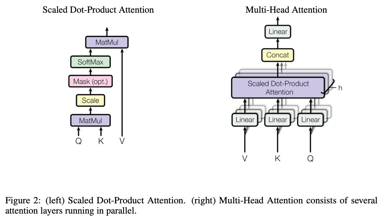
Scaled Dot-Product Attention:
The input consists of queries and keys of dimension dk, and values of dimension dv. We compute the dot products of the query with all keys, divide each by pdk, and apply a softmax function to obtain the weights on the values.
In practice, we compute the attention function on a set of queries simultaneously, packed together into a matrix Q. The keys and values are also packed together into matrices K and V . We compute the matrix of outputs as:
X ∈ (len, dmodel), WQ ∈ (dmodel, dk), WK ∈ (dmodel, dk), WV ∈ (dmodel, dv)
Q = X * WQ ∈ (len, dk)
K = X * WK ∈ (len, dk)
V = X * WV ∈ (len, dv)
Q * K.T ∈ (len, len)
softmax(Q * K.T / √dk) ∈ (len, len)
softmax(Q * K.T / √dk) * V ∈ (len, dv)
two types of attention: additive attention and dot-product attention?
Why divide √dk?
- And the author suspect for large values of dk, the dot products grow large in magnitude, pushing the softmax function into regions where it has extremely small gradients
- q · k = sum(qi * ki) for i from 1 to dk, has mean 0 and variance dk.
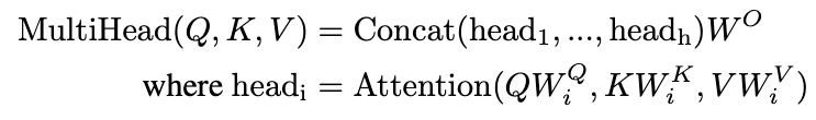
Multi-Head Attention:
We found it beneficial to linearly project the queries, keys and values h times with different, learned
linear projections to dk, dk and dv dimensions, respectively.
On each of these projected versions of queries, keys and values we then perform the attention function in parallel, yielding dv-dimensional output values(len*dv). These are concatenated and once again projected, resulting in the final values, as depicted in Figure:
The Q, K, V should be the output of previous layer, the shape is (len, dmodel)
headi ∈ (len, dv), WO ∈ (h * dv, dmodel)
MultiHead(Q, K, V) ∈ (len, dmodel)
the author uses h = 8, dk = dv = dmodel/h = 64, dmodel = 512
In implemention, we combine the h head in one linear layer as:
X ∈ (len, dmodel), WQ ∈ (dmodel, h * dk), WK ∈ (dmodel, h * dk), WV ∈ (dmodel, h * dv)
h * dk = dmodel
Q = X * WQ ∈ (len, h * dk)
K = X * WK ∈ (len, h * dk)
V = X * WV ∈ (len, h * dv)
Q * K.T ∈ (len, len)
softmax(Q * K.T / √dk) ∈ (len, len)
softmax(Q * K.T / √dk) * V ∈ (len, h * dv)
1 | # querys -> (B, len, d_k) |
Applications of Attention in our Model:
- In a self-attention in encoder, the Q, K, V comes from previous layer’s output
- In the attention in decoder, the Q comes from the previous decoder, and K, V comes from encoder.
- In decoder, when we predict word i, we mask out (setting to −∞) all work i+1 to len in K, V from encoder.
Position-wise Feed-Forward Networks
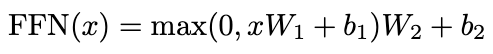
X ∈ (len, dmodel), W1 ∈ (dmodel, dff), W1 ∈ (dff, dmodel), b ∈ (len, dmodel)
X * W1 ∈ (len, dff)
FFN(x) ∈ (len, dmodel)
dmodel = 512, dff = 2048
Embeddings and Softmax
In our model, we share the same weight matrix between the two embedding layers and the pre-softmax linear transformation(convert the decoder output to predicted next-token probabilities). In the embedding layers, we multiply those weights by √dmodel.
WHY?
Positional Encoding
In order for the model to make use of the order of the sequence, we must inject some information about the relative or absolute position of the tokens in the sequence.
We add “positional encodings” to the input embeddings at the bottoms of the encoder and decoder stacks. In this work, we use sine and cosine functions of different frequencies:
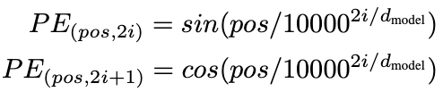
where pos is the position and i is the dimension, and any fixed offset k, PE(pos+k) can be represented as a linear function of PE(pos).
Why Self-Attention
We compare various aspects of self-attention layers to the recurrent and convolutional layers.
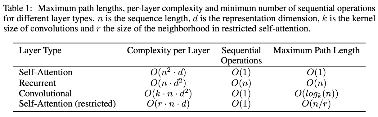
One is the total computational complexity per layer.
In terms of computational complexity, self-attention layers are faster than recurrent layers when the sequence length n is smaller than the representation dimensionality d.
To improve computational performance for tasks involving very long sequences, self-attention could be restricted to considering only a neighborhood of size r in the input sequence centered around the respective output position. This would increase the maximum path length to O(n/r).
A single convolutional layer with kernel width k < n does not connect all pairs of input and output positions. Doing so requires a stack of O(n/k) convolutional layers in the case of contiguous kernels, or O(logk(n)) in the case of dilated convolutions. Convolutional layers are generally more expensive than recurrent layers, by a factor of k.
Another is the amount of computation that can be parallelized.
The third is the path length between long-range dependencies in the network.
Learning long-range dependencies is a key challenge in many sequence transduction tasks. One key factor affecting the ability to learn such dependencies is the length of the paths forward and backward signals have to traverse in the network. The shorter these paths between any combination of positions in the input and output sequences, the easier it is to learn long-range dependencies.
GPT
Labeled data for learning these specific tasks is scarce, so it is challenging for discriminatively trained models to perform adequately.
We demonstrate that large gains on these tasks can be realized by generative pre-training of a language model on a diverse corpus of unlabeled text, followed by discriminative fine-tuning on each specific task.
Introduction
Models that can leverage linguistic information from unlabeled data provide a valuable alternative to gathering more annotation, which can be time-consuming and expensive. Further, even in cases where considerable supervision is available, learning good representations in an unsupervised fashion can provide a significant performance boost.
Leveraging more than word-level information from unlabeled text, however, is challenging for two main reasons.
- It is unclear what type of optimization objectives are most effective at learning text representations that are useful for transfer.
- There is no consensus on the most effective way to transfer these learned representations to the target task.
In this paper, we explore a semi-supervised approach for language understanding tasks using a combination of unsupervised pre-training and supervised fine-tuning.
Our goal is to learn a universal representation that transfers with little adaptation to a wide range of tasks.
We employ a two-stage training procedure:
- First, we use a language modeling objective on the unlabeled data to learn the initial parameters of a neural network model.
- Subsequently, we adapt these parameters to a target task using the corresponding supervised objective.
For our model architecture, we use the Transformer.
During transfer, we utilize task-specific input adaptations derived from traversal-style approaches, which process structured text input as a single contiguous sequence of tokens.
Related Work
Semi-supervised learning for NLP
The earliest approaches used unlabeled data to compute word-level or phrase-level statistics. Over the last few years, researchers have demonstrated the benefits of using word embeddings.
These approaches, however, mainly transfer word-level information, whereas we aim to capture higher-level semantics.
Unsupervised pre-training
Research demonstrated that pre-training acts as a regularization scheme, enabling better generalization in deep neural networks.
The usage of LSTM models in other approaches restricts their prediction ability to a short range. Our choice of transformer networks allows us to capture longerrange linguistic structure.
Other approaches use hidden representations from a pre-trained model involving a substantial amount of new parameters for each separate target task, whereas we require minimal changes to our model architecture during transfer.
Auxiliary training objectives
POS tagging, chunking, named entity recognition, and language modeling.
Framework
Our training procedure consists of two stages. The first stage is learning a high-capacity language
model on a large corpus of text. This is followed by a fine-tuning stage, where we adapt the model to
a discriminative task with labeled data.
Unsupervised pre-training
We use a standard language modeling objective to maximize the following likelihood:
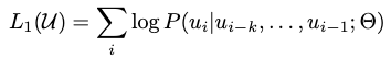
where k is the size of the context window, and the conditional probability P is modeled using a neural network with parameters Θ. These parameters are trained using stochastic gradient descent.
In our experiments, we use a multi-layer Transformer decoder or the language model, which is a variant of the transformer. This model applies a multi-headed self-attention operation over the input context tokens followed by position-wise feedforward layers to produce an output distribution over target tokens:
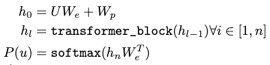
where U = (u−k, … , u−1) is the context vector of tokens, n is the number of layers, We is the token
embedding matrix, and Wp is the position embedding matrix.
Supervised fine-tuning
We assume a labeled dataset C, where each instance consists of a sequence of input tokens, x1, … , xm, along with a label y.
The inputs are passed through our pre-trained model to obtain the final transformer block’s activation h(m,l) , which is then fed into an added linear output layer with parameters Wy to predict y:
This gives us the following objective to maximize:
Specifically, we optimize the following objective (with weight λ):

Overall, the only extra parameters we require during fine-tuning are Wy , and embeddings for delimiter tokens.
Task-specific input transformations
Certain other tasks, like question answering or textual entailment, have structured inputs such as ordered sentence pairs, or triplets of document, question, and answers.
Since our pre-trained model was trained on contiguous sequences of text, we require some modifications to apply it to these tasks.
we use a traversal-style approach [52], where we convert structured inputs into an ordered sequence that our pre-trained model can process. These input transformations allow us to avoid making extensive changes to the architecture across tasks.
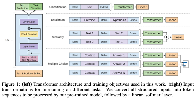
All transformations include adding randomly initialized start and end tokens (⟨s⟩, ⟨e⟩).
Textual entailment
Similarity
Question Answering and Commonsense Reasoning
Bert
BERT, which stands for Bidirectional Encoder Representations from Transformers.
BERT is designed to pretrain deep bidirectional representations from unlabeled text by jointly conditioning on both left and right context in all layers.
Introduction
Language model pre-training has been shown to be effective for improving many natural language processing tasks.
There are two existing strategies for applying pre-trained language representations to downstream tasks: feature-based and fine-tuning.
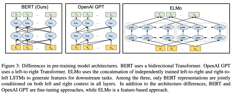
The feature-based approach, such as ELMo, uses task-specific architectures that include the pre-trained representations as additional features.
The fine-tuning approach, such as the Generative Pre-trained Transformer (OpenAI GPT) (Radford et al., 2018), introduces minimal task-specific parameters, and is trained on the downstream tasks by simply fine-tuning all pretrained parameters.
We argue that current techniques restrict the power of the pre-trained representations, especially for the fine-tuning approaches.
The major limitation is that standard language models are unidirectional, and this limits the choice of architectures that can be used during pre-training. For example, in OpenAI GPT, the authors use a left-to-right architecture, where every token can only attend to previous tokens in the self-attention layers of the Transformer.
In this paper, we improve the fine-tuning based approaches by proposing BERT: Bidirectional Encoder Representations from Transformers. BERT alleviates the previously mentioned unidirectionality constraint by using a “masked language model” (MLM) pre-training objective.
The masked language model randomly masks some of the tokens from the input, and the objective is to predict the original vocabulary id of the masked word based only on its context.
Unlike left-to-right language model pre-training, the MLM objective enables the representation to fuse the left and the right context, which allows us to pretrain a deep bidirectional Transformer.
In addition to the masked language model, we also use a “next sentence prediction” task that jointly pretrains text-pair representations.
Related Work
Unsupervised Feature-based Approaches
Pre-trained word embeddings are an integral part of modern NLP systems, offering significant improvements over embeddings learned from scratch.
ELMo and its predecessor generalize traditional word embedding research along a different dimension. They extract context-sensitive features from a left-to-right and a right-to-left language model.
Unsupervised Fine-tuning Approaches
More recently, sentence or document encoders which produce contextual token representations have been pre-trained from unlabeled text and fine-tuned for a supervised downstream task.
The advantage of these approaches is that few parameters need to be learned from scratch.
At least partly due to this advantage, OpenAI GPT (Radford et al., 2018) achieved previously state-of-the-art results on many sentence-level tasks from the GLUE benchmark.
Transfer Learning from Supervised Data
BERT
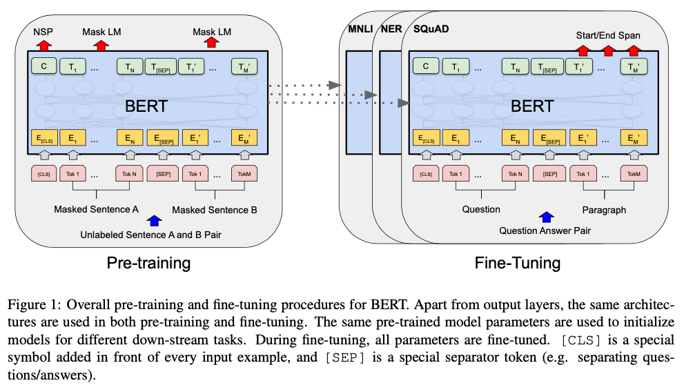
There are two steps in our framework: pre-training and fine-tuning.
During pre-training, the model is trained on unlabeled data over different pre-training tasks. For fine-tuning, the BERT model is first initialized with the pre-trained parameters, and all of the parameters are fine-tuned using labeled data from the downstream tasks.
A distinctive feature of BERT is its unified architecture across different tasks. There is minimal difference between the pre-trained architecture and the final downstream architecture.
Model Architecture
BERT’s model architecture is a multi-layer bidirectional Transformer encoder.
In this work, we denote the number of layers (i.e., Transformer blocks) as L, the hidden size as H, and the number of self-attention heads as A.
We primarily report results on two model sizes: BERT(BASE) (L=12, H=768, A=12, Total Parameters=110M) and BERT(LARGE) (L=24, H=1024, A=16, Total Parameters=340M).
In all cases we set the feed-forward/filter size to be 4H, i.e., 3072 for the H = 768 and 4096 for the H = 1024.
BERT(BASE) was chosen to have the same model size as OpenAI GPT for comparison purposes. Critically, however, the BERT Transformer uses bidirectional self-attention, while the GPT Transformer uses constrained self-attention where every token can only attend to context to its left.
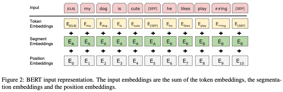
Input/Output Representations
To make BERT handle a variety of down-stream tasks, our input representation is able to unambiguously represent both a single sentence and a pair of sentences (e.g., ⟨ Question, Answer ⟩) in one token sequence.
A “sequence” refers to the input token sequence to BERT, which may be a single sentence or two sentences packed together.
We use WordPiece embeddings (Wu et al., 2016) with a 30,000 token vocabulary.
The first token of every sequence is always a special classification token ([CLS]).
Sentence pairs are packed together into a single sequence. We differentiate the sentences in two ways. First, we separate them with a special token ([SEP]). Second, we add a learned embedding to every token indicating whether it belongs to sentence A or sentence B.
C ∈ (H,), Ti ∈ (H,)
Pre-training BERT
We pre-train BERT using two unsupervised tasks, described in this section.
Task #1: Masked LM
Intuitively, it is reasonable to believe that a deep bidirectional model is strictly more powerful than either a left-to-right model or the shallow concatenation of a left-to-right and a right-to-left model.
Unfortunately, standard conditional language models can only be trained left-to-right or right-to-left, since bidirectional conditioning would allow each word to indirectly “see itself”, and the model could trivially predict the target word in a multi-layered context.
In order to train a deep bidirectional representation, we simply mask some percentage of the input tokens at random, and then predict those masked tokens.
In this case, the final hidden vectors corresponding to the mask tokens are fed into an output softmax over the vocabulary, as in a standard LM. We refer to this procedure as a “masked LM” (MLM).
In all of our experiments, we mask 15% of all WordPiece tokens in each sequence at random. In contrast to denoising auto-encoders, we only predict the masked words rather than reconstructing the entire input.
A downside is that we are creating a mismatch between pre-training and fine-tuning, since the [MASK] token does not appear during fine-tuning.
To mitigate this, we chooses 15% of the token positions at random for prediction. If the i-th token is chosen, we replace the i-th token with (1) the [MASK] token 80% of the time (2) a random token 10% of the time (3) the unchanged i-th token 10% of the time.
Then, Ti will be used to predict the original token with cross entropy loss.
Task #2: Next Sentence Prediction (NSP)
In order to train a model that understands sentence relationships, we pre-train for a binarized next sentence prediction task that can be trivially generated from any monolingual corpus.
Specifically, when choosing the sentences A and B for each pre- training example, 50% of the time B is the actual next sentence that follows A (labeled as IsNext), and 50% of the time it is a random sentence from the corpus (labeled as NotNext).
As we show in Figure 1, C is used for next sentence prediction (NSP).
Pre-training data
For the pre-training corpus we use the BooksCorpus (800M words) and English Wikipedia (2,500M words). It is criti- cal to use a document-level corpus rather than a shuffled sentence-level corpus in order to extract long contiguous sequences.
Fine-tuning BERT
For each task, we simply plug in the task-specific inputs and outputs into BERT and fine-tune all the parameters end-to-end.
At the output, the token representations are fed into an output layer for token-level tasks, such as sequence tagging or question answering, and the [CLS] representation is fed into an output layer for classification, such as entailment or sentiment analysis.
Compared to pre-training, fine-tuning is relatively inexpensive.