Overview
- Parallelism
- Model parallelism
- Data parallelism
- Synchronous vs asynchronous training
- TensorFlow Strategy
- Model Computation Pipelining
- Graph optimization with Grappler
- MetaOptimizer
- Pruning optimizer
- Function optimizer
- Common subgraph elimination
- Debug stripper
- Constant folding optimizer
- Shape optimizer
- Auto mixed precision optimizer
- Pin to host optimizer
- Arithmetic optimizer
- Layout optimizer
- Remapper optimizer
- Loop optimizer
- Dependency optimizer
- Memory optimizer
- Autoparallel optimizer
- Scoped allocator optimizer
- Distributed architecture (unfinished)
- Parameter server
- Ring-allreduce
- Horovod
1 Parallelism
TensorFlow’s basic dataflow graph model can be used in a variety of ways for machine learning applications. However, some neural networks models are so large they cannot fit in memory of a single device (GPU). Google’s Neural Machine Translation system is an example of such a network.
Such models need to be split over many devices, carrying out the training in parallel on the devices. There are three method to train a model in parallel on the devices, Model parallelism, Data parallelism, and Model Computation Pipelining.
Model parallelism uses same data for every device but partitions the model among the devices. The graph is split as several sub-graphs, and assigns these sub-graphs to feasible devices to training. All devices use a same mini-batch to train.
Data parallelism uses the same model for every device, but train the model in each device using different training samples. Each device holds a entire model, but trains with partial samples from the mini-batch.
Model Computation Pipelining pipelines the computation of seveal same models within one device by running a small number of concurrent steps.
1.1 Model parallelism
Model parallel training, where different portions of the model computation are done on different computational devices simultaneously for the same batch of examples, as the following figure:
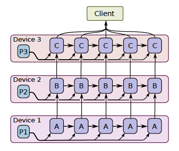
It is challenging to get good performance, because some layers may depend on previous layers which leads to a long waiting time. However, if a model has some components which can run in parallel, it can use this method to improve the efficiency.
1.2 Data parallelism
In modern deep learning, because the dataset is too big to be fit into the memory, we could only do stochastic gradient descent(SGD) for batches. The shortcoming of SGD is that the estimate of the gradients might not accurately represent the true gradients of using the full dataset. Therefore, it may take much longer to converge.
Data parallelism is a simple technique for speeding up SGD is to parallelize the computation of the gradient for a mini-batch across devices.
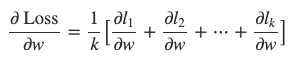
Each device will independently compute the loss the gradients of small batches, the final estimate of the gradients is the weighted average of the gradients calculated from all the small batches(require communication).
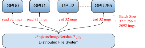
By using data parallelism, the model can train on a large batch size. For example, the folloing figure shows a typical data parallelism, distributing 32 different images to each of the 256 GPUs running a single model. Together, the total mini-batch size for an iteration is 8,092 images (32 x 256) (Facebook: Training ImageNet in 1 Hour).
Mathematically, data parallelism is valid because:
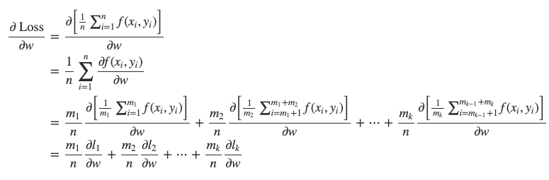
* m1+m2+⋯+mk=n.
When m1=m2=⋯=mk=nk, we could further have:
1.2.1 Synchronous vs asynchronous training
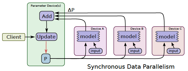
In synchronous training(as following figure), all of the devices train their local model using different parts of data from a single (large) mini-batch. They then communicate their locally calculated gradients (directly or indirectly) to all devices.
Only after all devices have successfully computed and sent their gradients is the model updated. The updated model is then sent to all nodes along with splits from the next mini-batch. That is, devices train on non-overlapping splits (subset) of the mini-batch.
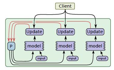
In asynchronous training, no device waits for updates to the model from any other device. The devices can run independently and share results as peers, or communicate through one or more central servers known as “parameter” servers.
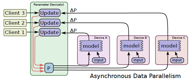
In synchronous training, the parameter servers compute the latest up-to-date version of the model, and send it back to devices. In asynchronous training, parameter servers send gradients to devices that locally compute the new model.
1.2.2 TensorFlow Strategy
tf.distribute.Strategy is a TensorFlow API to distribute training across multiple GPUs, multiple machines or TPUs. Using this API.
It intends to cover a number of use cases along different axes, including:
- synchronous vs asynchronous training,
- hardware platform(multiple GPUs on one machine, or multiple machines in a network, or on Cloud TPUs).
MirroredStrategy
tf.distribute.MirroredStrategy supports synchronous distributed training on multiple GPUs on one machine.
It creates one replica per GPU device. During training, one mini-batch is split into N parts and each part feed to one GPU device.
Efficient all-reduce algorithms are used to communicate the variable updates across the devices. By default, it uses NVIDIA NCCL as the all-reduce implementation. Currently, tf.distribute.HierarchicalCopyAllReduce and tf.distribute.ReductionToOneDevice are two options other than tf.distribute.NcclAllReduce which is the default.
CentralStorageStrategy
tf.distribute.experimental.CentralStorageStrategy does synchronous training as well. Variables are not mirrored, instead they are placed on the CPU and operations are replicated across all local GPUs. If there is only one GPU, all variables and operations will be placed on that GPU.
MultiWorkerMirroredStrategy
tf.distribute.experimental.MultiWorkerMirroredStrategy is very similar to MirroredStrategy. It implements synchronous distributed training across multiple workers, each with potentially multiple GPUs. Similar to MirroredStrategy, it creates copies of all variables in the model on each device across all workers.
It uses CollectiveOps as the multi-worker all-reduce communication method used to keep variables in sync.
A collective op is a single op in the TensorFlow graph which can automatically choose an all-reduce algorithm in the TensorFlow runtime according to hardware, network topology and tensor sizes.
MultiWorkerMirroredStrategy currently allows two different implementations of collective ops:
- CollectiveCommunication.RING, ring algorithms for all-reduce and all-gather.
- CollectiveCommunication.NCCL, ncclAllReduce for all-reduce, and ring algorithms for all-gather.
TPUStrategy
tf.distribute.experimental.TPUStrategy lets you run your TensorFlow training on Tensor Processing Units (TPUs).
ParameterServerStrategy
tf.distribute.experimental.ParameterServerStrategy supports parameter servers training on multiple machines. In this setup, some machines are designated as workers and some as parameter servers. Each variable of the model is placed on one parameter server. Computation is replicated across all GPUs of all the workers.
OneDeviceStrategy
tf.distribute.OneDeviceStrategy runs on a single device. This strategy will place any variables created in its scope on the specified device. Input distributed through this strategy will be prefetched to the specified device.
You can use this strategy to test your code before switching to other strategies which actually distributes to multiple devices/machines.
1.3 Model Computation Pipelining
Another common way to get better utilization for training deep neural networks is to pipeline the computation of the model within the same devices, by running a small number of concurrent steps within the same set of devices.
It is somewhat similar to asynchronous data parallelism, except that the parallelism occurs within the same device(s), rather than replicating the computation graph on different devices.
This allows “filling in the gaps” where computation of a single batch of examples might not be able to fully utilize the full parallelism on all devices at all times during a single step.
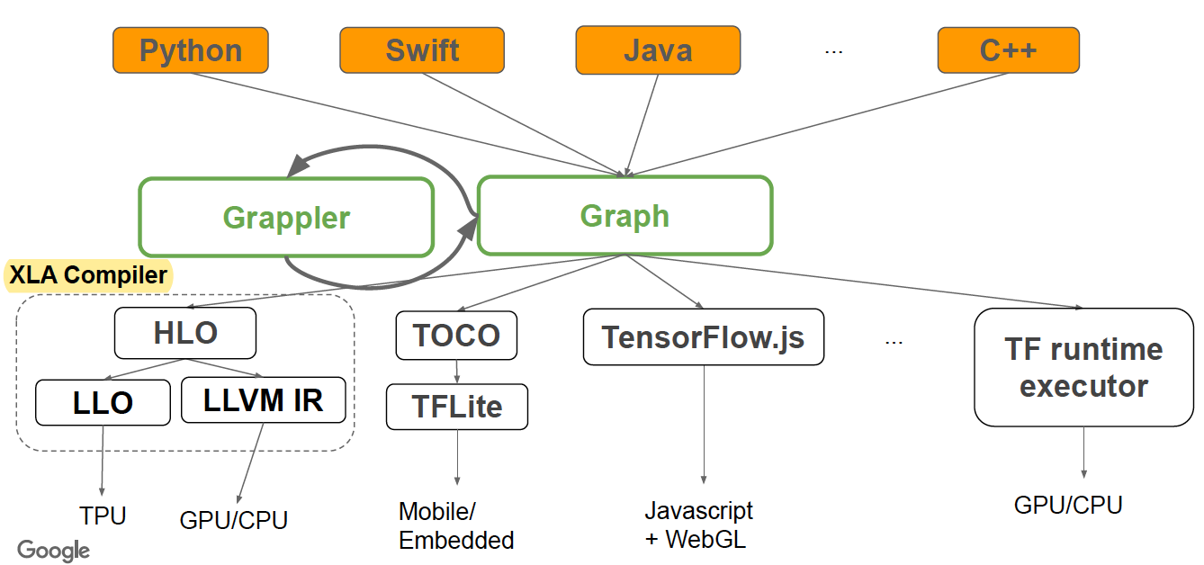
2 Graph optimization with Grappler
Graph is the default graph optimization system in the TF runtime to:
- Automatically improve TF performance through graph simplifications & high-level optimizations
- Reduce device peak memory usage to enable larger models to run
- Improve hardware utilization by optimizing the mapping of graph nodes to compute resources
2.1 MetaOptimizer
MetaOptimizer is the top-level driver invoked by runtime or standalone tool, it Runs multiple sub-optimizers in a loop: (* = not on by default):
1 | i = 0 |
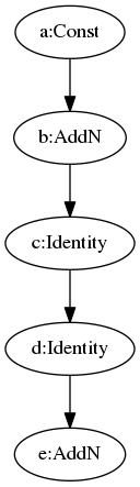
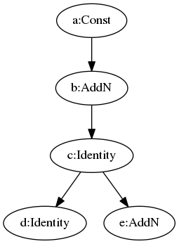
2.2 Pruning optimizer
Prunes nodes that have no effect on the output from the graph. It is usually run first to reduce the size of the graph and speed up processing in other Grappler passes.
Typically, this optimizer removes some StopGradient nodes and Identity nodes. For example, as the folloing figure, the Identity node is moved to a new branch.
 |
 |
2.3 Function optimizer
Optimizes the function library of a TensorFlow program and inlines function bodies to enable other inter-procedural optimizations.
2.4 Common subgraph elimination
This optimizer travels the entire graph to find and dedup same subgraphs.
2.5 Debug stripper
Strips nodes related to debugging operations such as tf.debugging.Assert, tf.debugging.check_numerics, and tf.print from the graph.
This optimizer is turned OFF by default.
2.6 Constant folding optimizer
Statically infers the value of tensors when possible by folding constant nodes in the graph and materializes the result using constants.
This optimizer has three methods: MaterializeShapes, FoldGraph, and SimplifyGraph.
MaterializeShapes handles three nodes: Shape, Size, and Rank. Because these three nodes depend on the shape of input tensor, so it doesn’t have relationship with the value of the tensor. MaterializeShapes replaces these three node with Const node.
FoldGraph folds the node whose all inputs are Const node, because its output can be pre-computed.
SimplifyGraph handles:
- Constant push-down:
- Add(c1, Add(x, c2)) => Add(x, c1 + c2)
- ConvND(c1 * x, c2) => ConvND(x, c1 * c2)
- Partial constfold:
- AddN(c1, x, c2, y) => AddN(c1 + c2, x, y),
- Concat([x, c1, c2, y]) = Concat([x, Concat([c1, c2]), y)
- Operations with neutral & absorbing elements:
- x * Ones(s) => Identity(x), if shape(x) == output_shape
- x * Ones(s) => BroadcastTo(x, Shape(s)), if shape(s) == output_shape
- Same for x + Zeros(s) , x / Ones(s), x * Zeros(s) etc.
- Zeros(s) - y => Neg(y), if shape(y) == output_shape
- Ones(s) / y => Recip(y) if shape(y) == output_shape
2.7 Shape optimizer
Optimizes subgraphs that operate on shape and shape related information.
2.8 Auto mixed precision optimizer
Converts data types to float16 where applicable to improve performance. Currently applies only to GPUs.
2.9 Pin to host optimizer
Swaps small operations onto the CPU.
This optimizer is turned OFF by default.
2.10 Arithmetic optimizer
Simplifies arithmetic operations by eliminating common subexpressions and simplifying arithmetic statements.
- Arithmetic simplifications
- Flattening: a+b+c+d => AddN(a, b, c, d)
- Hoisting: AddN(x * a, b * x, x * c) => x * AddN(a+b+c)
- Simplification to reduce number of nodes:
- Numeric: x+x+x => 3*x
- Logic: !(x > y) => x <= y
- Broadcast minimization
- Example: (matrix1 + scalar1) + (matrix2 + scalar2) => (matrix1 + matrix2) + (scalar1 + scalar2)
- Better use of intrinsics
- Matmul(Transpose(x), y) => Matmul(x, y, transpose_x=True)
- Remove redundant ops or op pairs
- Transpose(Transpose(x, perm), inverse_perm)
- BitCast(BitCast(x, dtype1), dtype2) => BitCast(x, dtype2)
- Pairs of elementwise involutions f(f(x)) => x (Neg, Conj, Reciprocal, LogicalNot)
- Repeated Idempotent ops f(f(x)) => f(x) (DeepCopy, Identity, CheckNumerics…)
- Hoist chains of unary ops at Concat/Split/SplitV
- Concat([Exp(Cos(x)), Exp(Cos(y)), Exp(Cos(z))]) => Exp(Cos(Concat([x, y, z])))
- [Exp(Cos(y)) for y in Split(x)] => Split(Exp(Cos(x), num_splits)
2.11 Layout optimizer
Optimizes tensor layouts to execute data format dependent operations such as convolutions more efficiently.
For some nodes including AvgPool, Conv2D, etc, they supports two types of input format, NHWC and NCHW. But at the GPU runtime kernel, the NCHW data foramt is more efficient. This optimize adds a node to transfer the data format before these nodes.
For example, the following original graph with all ops in NHWC format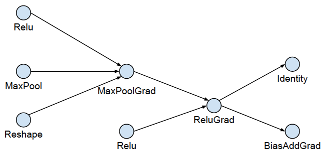
Phase 1, expand by inserting conversion pairs: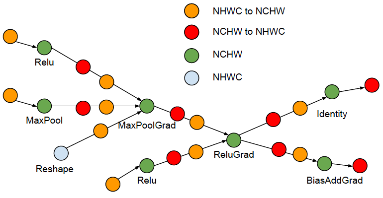
Phase 2, collapse adjacent conversion pairs: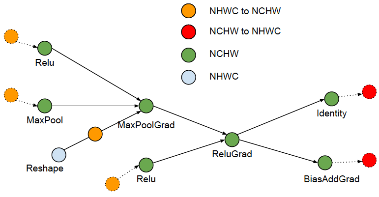
This optimizer only runs at the first iteration.
2.12 Remapper optimizer
Remaps subgraphs onto more efficient implementations by replacing commonly occuring subgraphs with optimized fused monolithic kernels.
Replaces commonly occurring subgraphs with optimized fused “monolithic” kernels:
- Conv2D + BiasAdd + <Activation>
- Conv2D + FusedBatchNorm + <Activation>
- Conv2D + Squeeze + BiasAdd
- MatMul + BiasAdd + <Activation>
Several performance advantages:
- Completely eliminates Op scheduling overhead
- Improves temporal and spatial locality of data access
- E.g. MatMul is computed block-wise and bias and activation function can be
applied while data is still “hot” in cache
2.13 Loop optimizer
Optimizes the graph control flow by hoisting loop-invariant subgraphs out of loops and by removing redundant stack operations in loops. Also optimizes loops with statically known trip counts and removes statically known dead branches in conditionals.
- Loop Invariant Node Motion
1
2
3
4
5
6
7
8
9
10
for (int i = 0; i < n; i++) {
x = y + z;
a[i] = 6 * i + x * x;
}
// Motion the y+z and x*x
x = y + z;
t1 = x * x;
for (int i = 0; i < n; i++) {
a[i] = 6 * i + t1;
} - StackPush removal
- Remove StackPushes without consumers
- Dead Branch Elimination
- Deduce loop trip count statically
- Remove loop for zero trip count
- Remove control flow nodes for trip count == 1
2.14 Dependency optimizer
Removes or rearranges control dependencies to shorten the critical path for a model step or enables other optimizations. Also removes nodes that are effectively no-ops such as Identity.
A control edge is redundant iff there exists a path of length > 1 from source to control target: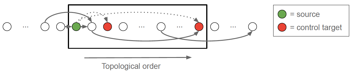
2.15 Memory optimizer
Analyzes the graph to inspect the peak memory usage for each operation and inserts CPU-GPU memory copy operations for swapping GPU memory to CPU to reduce the peak memory usage.
Memory optimization based on abstract interpretation
- Swap-out / Swap-in optimization
- Reduces device memory usage by swapping to host memory
- Uses memory cost model to estimate peak memory
- Uses op cost model to schedule Swap-In at (roughly) the right time
- Recomputation optimization (not on by default)
Peak Memory Characterization: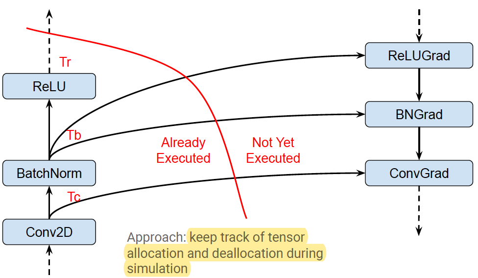
Swapping (start early):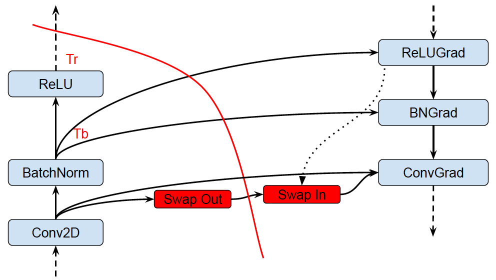
Recomputation: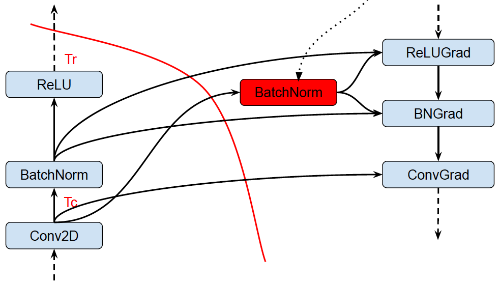
This optimizer only runs at the first iteration.
2.16 Autoparallel optimizer
Automatically parallelizes graphs by splitting along the batch dimension.
AutoParallel is similar to the MirroredStrategy, however, the AutoParallel implements the parallel training by modifying the graph, instead of using replicated mulitiply models.
For example, the following graph shows a graph, the Dequeue node fetches some samples from the FIFO node, add with Const node and as the input of ApplyGradient node whose logic is var −= add * learning_rate.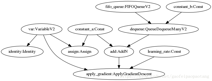
After applying AutoParallel with Replica=2, the following graph shows, some nodes keep same(FIFO), some nodes are duplicated(add, Dequeue), and some new nodes are added(Div).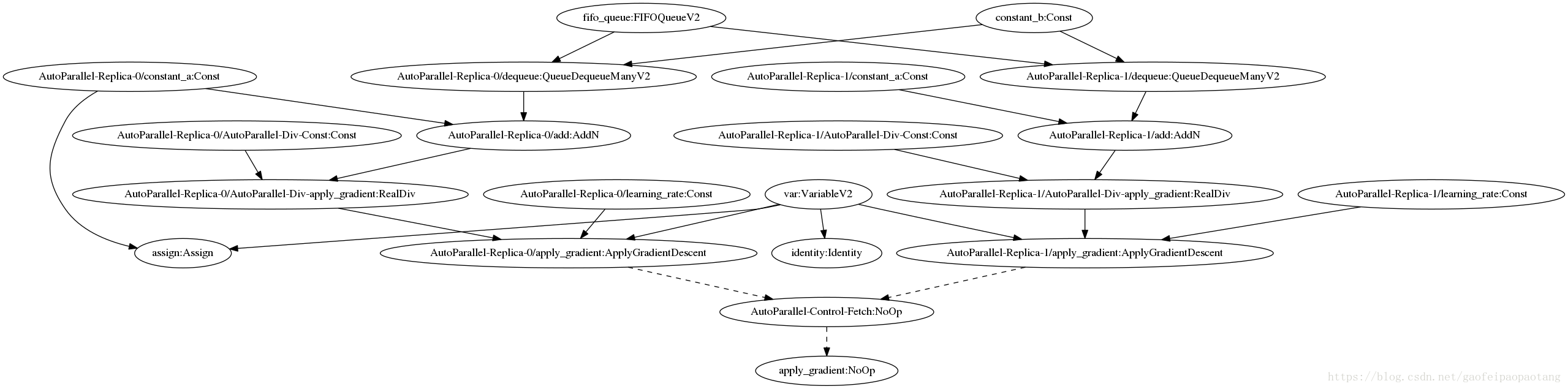
These two ApplyGradientDescent nodes can run parallelly to compute:
var −= add(replica−0)/2 * learning_rate(replica−0)
var −= add(replica−1)/2 * learning_rate(replica−1)
This optimizer is turned OFF by default.
2.17 Scoped allocator optimizer
Introduces scoped allocators to reduce data movement and to consolidate some operations.
This optimizer only runs at the last iteration.
3 Distributed architecture (unfinished)
Reference
- https://www.oreilly.com/content/distributed-tensorflow/
- https://www.tensorflow.org/guide/distributed_training
- https://www.tensorflow.org/guide/graph_optimization
- https://web.stanford.edu/class/cs245/slides/TFGraphOptimizationsStanford.pdf
- Abadi, M., Agarwal, A., Barham, P., Brevdo, E., Chen, Z., Citro, C., … & Ghemawat, S. (2016). Tensorflow: Large-scale machine learning on heterogeneous distributed systems. arXiv preprint arXiv:1603.04467.
- Sergeev, A., & Del Balso, M. (2018). Horovod: fast and easy distributed deep learning in TensorFlow. arXiv preprint arXiv:1802.05799.
- Abadi, M., Barham, P., Chen, J., Chen, Z., Davis, A., Dean, J., … & Kudlur, M. (2016). Tensorflow: A system for large-scale machine learning. In 12th {USENIX} Symposium on Operating Systems Design and Implementation ({OSDI} 16) (pp. 265-283).
- Mirhoseini, A., Pham, H., Le, Q. V., Steiner, B., Larsen, R., Zhou, Y., … & Dean, J. (2017, August). Device placement optimization with reinforcement learning. In Proceedings of the 34th International Conference on Machine Learning-Volume 70 (pp. 2430-2439). JMLR. org.
- https://leimao.github.io/blog/Data-Parallelism-vs-Model-Paralelism/
- Goyal, P., Dollár, P., Girshick, R., Noordhuis, P., Wesolowski, L., Kyrola, A., … & He, K. (2017). Accurate, large minibatch sgd: Training imagenet in 1 hour. arXiv preprint arXiv:1706.02677.
- https://github.com/tensorflow/tensorflow/blob/master/tensorflow/core/grappler/optimizers/meta_optimizer.cc